With machine-learning modeling, the team created the world’s highest-resolution brain tissue map.
This brain map lets researchers see 57,000 cells and 150 million synapses, which are connections between the neurons.
How are we ever going to really come to terms with all this complexity?
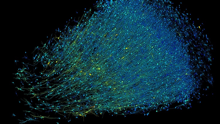
Photo: Google Research & Lichtman Lab (Harvard University)/Rendering by D. Berger (Harvard University)/CC4.0
The brain tissue comes from a 45-year-old woman who had undergone surgery to address her epilepsy.
Additionally, cadavers, which are often used in medical research, are not helpful because brains decompose quickly.
Those slices were then examined through an electron microscope made specifically for this study.
Rendering based on electron-microscope data, showing the positions of neurons in a fragment of the brain cortex. Neurons are colored according to size. (Photo: Google Research & Lichtman Lab (Harvard University)/Rendering by D. Berger (Harvard University)/CC4.0)
Rendering based on electron-microscope data, showing the positions of neurons in a fragment of the brain cortex.
Neurons are colored according to size.
Brain maps have been created before, starting in 1986 when 302 neurons were mapped in a roundworm.
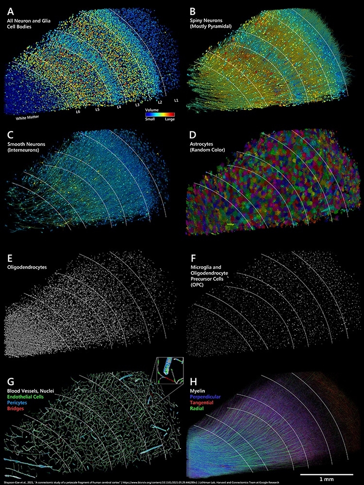
Distribution of cells, blood vessels and myelin in the sample. White lines in all panels indicate approximate layer boundaries estimated from cell clustering. A: All 49,080 manually labeled cell bodies of neurons and glia which were found in the sample, colored by cell body volume. B: All neurons classified as spiny cells (putatively excitatory), extracted from the C3-agglomerated. (Photo: Google Research & Lichtman Lab (Harvard University)/Rendering by D. Berger (Harvard University)/CC4.0)
If successful, a mapped mouse brain may give some insight into how humans learn and even free will.
Harvard and Google researchers published the most in-depth map of brain tissue to ever be created.
Distribution of cells, blood vessels and myelin in the sample.
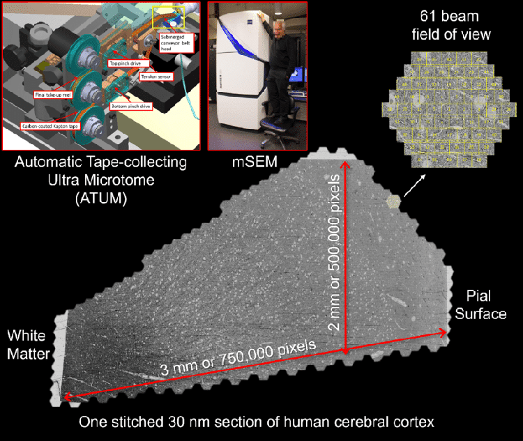
Image acquisition for the human brain sample. A fresh surgical cerebral cortex sample was rapidly preserved, then stained, embedded in resin, and sectioned. More than 5000 sequential ~30 nm sections were collected on tape using an ATUM (upper left panel). Yellow box shows the site where the brain sample is cut with the diamond knife and thin sections are collected onto the tape. The tape was then cut into strips and imaged in a multibeam scanning electron microscope (mSEM). This large machine (see middle panel with person on chair as reference) uses 61 beams that image a hexagonal area of about ~10,000 μm 2 simultaneously (see upper right). For each thin section, all the resulting tiles are then stitched together. One such stitched section is shown (bottom). This section is about 4 mm 2 in area and was imaged with 4 x 4 nm 2 pixels. Given the necessity of some overlap between the stitched tiles, this single section required collection of more than 300 GB of data.(Photo:GOOGLE RESEARCH & LICHTMAN LAB, HARVARD UNIVERSITY / D. BERGER (RENDERING)/CC4.0)
White lines in all panels indicate approximate layer boundaries estimated from cell clustering.
B: All neurons classified as spiny cells (putatively excitatory), extracted from the C3-agglomerated.
Image acquisition for the human brain sample.
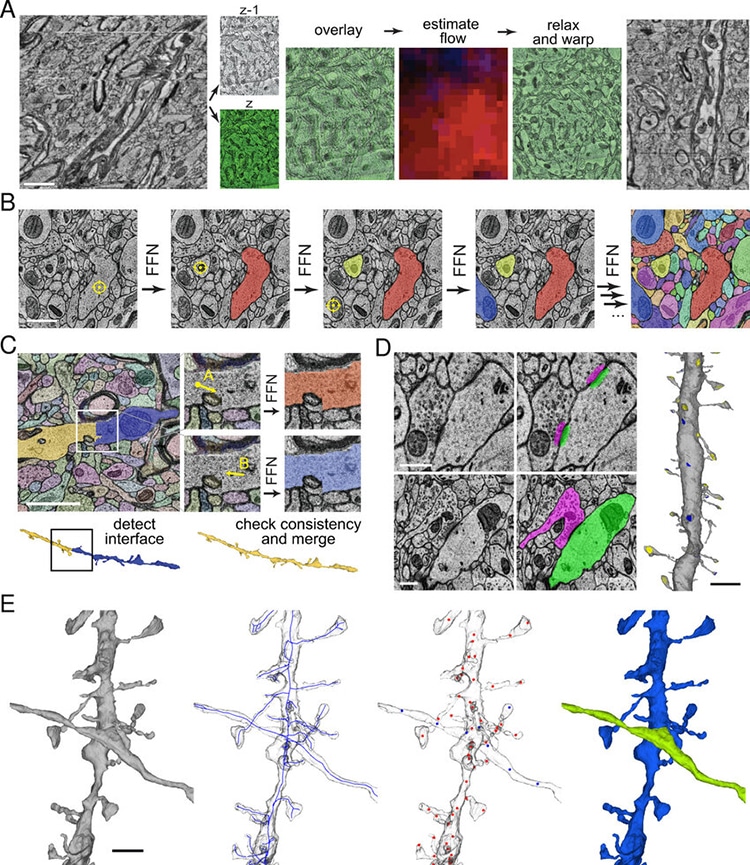
A: Fine-scale alignment with optical flow. Left: An XZ cross-section of the initial coarsely aligned subvolume exhibits drift and single-section jitter. Two adjacent XY sections z and z-1 are extracted. Center: z and z-1 are overlaid to illustrate their misalignment (z is pseudo-colored green for contrast). Image patch-based cross-correlation is used to compute an XY flow field between the sections. Red and blue intensity indicate the magnitude of the horizontal and vertical flow components respectively. The flow field is then used to warp one of the sections, improving the alignment apparent in the overlay. Right: XZ view of the same subvolume with flow realignment applied throughout. Scale bar: 2 μm. B: Sequential segmentation of a subvolume with an FFN. XY cross-sections illustrate the 3D segmentation process. Each yellow crosshair indicates the seed location for the next segment. Scale bar: 1 μm. C: FFN agglomeration.(Photo: Google Research & Lichtman Lab (Harvard University)/Rendering by D. Berger (Harvard University)/CC4.0)
A fresh surgical cerebral cortex sample was rapidly preserved, then stained, embedded in resin, and sectioned.
More than 5000 sequential ~30 nm sections were collected on tape using an ATUM (upper left panel).
The tape was then cut into strips and imaged in a multibeam scanning electron microscope (mSEM).
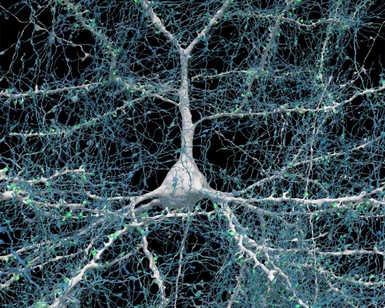
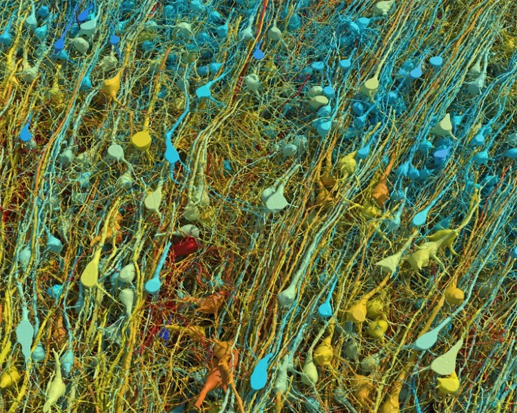
A single neuron (white) shown with 5,600 of the axons (blue) that connect to it. The synapses that make these connections are shown in green. (Photo: Google Research & Lichtman Lab (Harvard University)/Rendering by D. Berger (Harvard University)/CC4.0)
For each thin section, all the resulting tiles are then stitched together.
One such stitched section is shown (bottom).
This section is about 4 mm 2 in area and was imaged with 4 x 4 nm 2 pixels.
A: Fine-scale alignment with optical flow.
Left: An XZ cross-section of the initial coarsely aligned subvolume exhibits drift and single-section jitter.
Two adjacent XY sections z and z-1 are extracted.
Center: z and z-1 are overlaid to illustrate their misalignment (z is pseudo-colored green for contrast).
Image patch-based cross-correlation is used to compute an XY flow field between the sections.
Red and blue intensity indicate the magnitude of the horizontal and vertical flow components respectively.
Right: XZ view of the same subvolume with flow realignment applied throughout.
Scale bar: 2 m. B: Sequential segmentation of a subvolume with an FFN.
XY cross-sections illustrate the 3D segmentation process.
Each yellow crosshair indicates the seed location for the next segment.
Scale bar: 1 m. C: FFN agglomeration.
A single neuron (white) shown with 5,600 of the axons (blue) that connect to it.
The synapses that make these connections are shown in green.
